Part 3: SLAM & Autonomous Navigation

Introduction¶

Exercises: 3
Estimated Completion Time: 1 hour 30 minutes

Aims¶

From the work you did in Part 2 you may have started to appreciate the limitations associated with using odometry data alone as a feedback signal when trying to control a robot's position in its environment. In this next part you will explore an alternative data-stream that could be used to aid navigation further. You will leverage some existing ROS libraries and TurtleBot3 packages to explore some really powerful mapping and autonomous navigation methods that are available within ROS.

Intended Learning Outcomes¶

By the end of this session you will be able to:

Interpret the data that is published to the /scan topic and use existing ROS tools to visualise this.
Use existing ROS tools to implement SLAM and build a map of an environment.
Leverage existing ROS libraries to make a robot navigate an environment autonomously, using the map that you have generated.
Explain how these SLAM and Navigation tools are implemented and what information is required in order to make them work.

Quick Links¶

Exercise 1: Using RViz to Visualise Robot Data
Exercise 2: Building a map of an environment with SLAM
Exercise 3: Navigating an Environment Autonomously

Getting Started¶

Step 1: Launch your ROS Environment

If you haven't done so already, launch your ROS environment now:

Using WSL-ROS on a university managed desktop machine: follow the instructions here to launch it.
Running WSL-ROS on your own machine: launch the Windows Terminal to access a WSL-ROS terminal instance.
Other Users: Launch a terminal instance with access to your local ROS installation.

You should now have access to a Linux terminal instance, and we'll refer to this terminal instance as TERMINAL 1.

Step 2: Restore your work (WSL-ROS Managed Desktop Users ONLY)

Remember that any work that you do within the WSL-ROS Environment will not be preserved between sessions or across different University computers. At the end of Part 2 you should have run the wsl_ros tool to back up your home directory to your University U:\ Drive. Once WSL-ROS is up and running, you should be prompted to restore this:

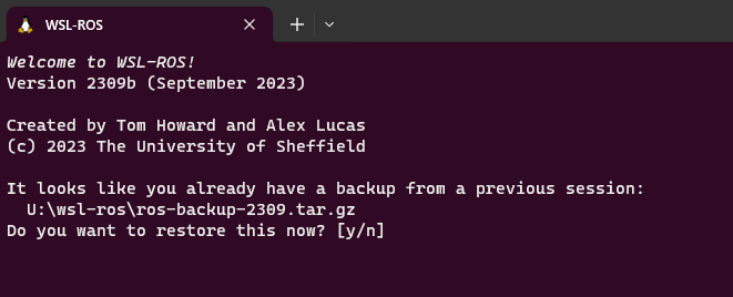
Enter Y to restore your work from last time. You can also restore your work at any time using the following command:

wsl_ros restore

Step 3: Launch VS Code

It's also worth launching VS Code now, so that it's ready to go for when you need it later on.

WSL Users...

It's important to launch VS Code within your ROS environment using the "WSL" extension. Always remember to check for this.

Step 4: Make Sure The Course Repo is Up-To-Date

In Part 1 you should have downloaded and installed The Course Repo into your ROS environment. Hopefully you've done this by now, but if you haven't then go back and do it now (you'll need it for some exercises here). If you have already done it, then (once again) it's worth just making sure it's all up-to-date, so run the following command now to do so:

TERMINAL 1:

roscd && cd ../src/tuos_ros/ && git pull

Then run catkin build

roscd && cd .. && catkin build

And finally, re-source your environment:

source ~/.bashrc

Remember

If you have any other terminal instances open, then you'll need run source ~/.bashrc in these too, in order for the changes made by catkin build to propagate through to these as well!

Laser Displacement Data and The LiDAR Sensor¶

As you'll know from Part 2, odometry is really important for robot navigation, but it can be subject to drift and accumulated error over time. You may have observed this in simulation during Part 2 Exercise 5, and you would most certainly notice it if you were to do the same on a real robot. Fortunately, our robots have another sensor on-board which provides even richer information about the environment, and we can use this to supplement the odometry information and enhance the robot's navigation capabilities.

Exercise 1: Using RViz to Visualise Robot Data¶

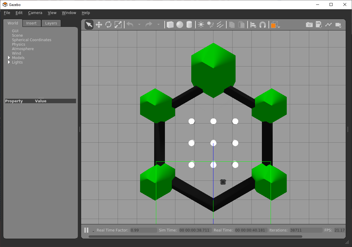
We're now going to place the robot in a more interesting environment than the "empty world" we've used in the previous parts of this course so far...

In TERMINAL 1 enter the following command to launch this:

TERMINAL 1:
```
roslaunch turtlebot3_gazebo turtlebot3_world.launch
```
A Gazebo simulation should now be launched with a TurtleBot3 Waffle in a new environment:
Open a new terminal instance (TERMINAL 2) and enter the following:

TERMINAL 2:
```
roslaunch tuos_simulations rviz.launch
```
On running the command a new window should open:

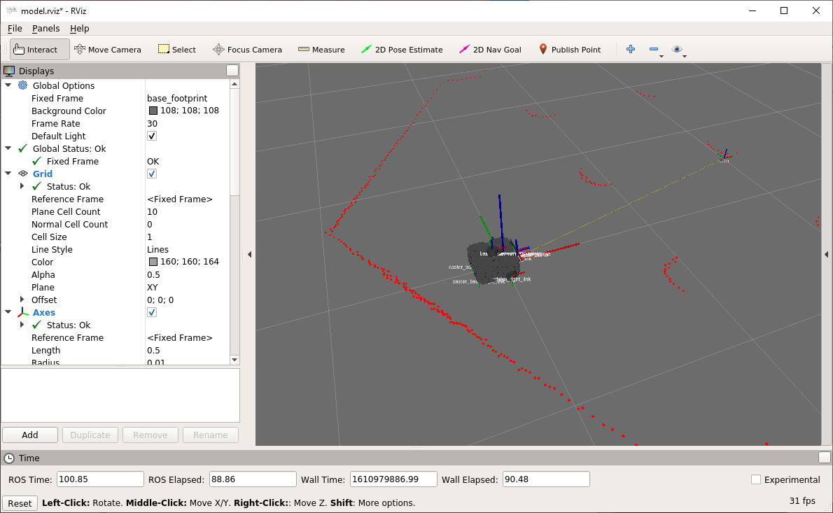
This is RViz, which is a ROS tool that allows us to visualise the data being measured by a robot in real-time. The red dots scattered around the robot represent laser displacement data which is measured by the LiDAR sensor located on the top of the robot. This data allows the robot to measure the distance to any obstacles in its immediate surroundings. The LiDAR sensor spins continuously, sending out laser pulses as it does so. These laser pulses then bounce off any objects and are reflected back to the sensor. Distance can then be determined based on the time it takes for the pulses to complete the full journey (from the sensor, to the object, and back again), by a process called "time of flight". Because the LiDAR sensor spins and performs this process continuously, a full 360° scan of the environment can be generated. In this case (because we are working in simulation here) the data represents the objects surrounding the robot in its simulated environment, so you should notice that the red dots produce an outline that resembles the objects in the world that is being simulated in Gazebo (or partially at least).
Next, open up a new terminal instance (TERMINAL 3). Laser displacement data from the LiDAR sensor is published by the robot to the /scan topic. We can use the rostopic info command to find out more about the nodes that are publishing and subscribing to this topic, as well as the message type:

TERMINAL 3:
```
rostopic info /scan
```
```
Type: sensor_msgs/LaserScan

Publishers:
    * /gazebo (http://localhost:#####/)

Subscribers:
    * /rviz_#### (http://localhost:#####/) 
```

As we can see from above, /scan messages are of the sensor_msgs/LaserScan type, and we can find out more about this message type using the rosmsg info command:

TERMINAL 3:

rosmsg info sensor_msgs/LaserScan

std_msgs/Header header
  uint32 seq
  time stamp
  string frame_id
float32 angle_min
float32 angle_max
float32 angle_increment
float32 time_increment
float32 scan_time
float32 range_min
float32 range_max
float32[] ranges
float32[] intensities

Interpreting `/LaserScan` Data¶

The LaserScan message is a standardised ROS message (from the sensor_msgs package) that any ROS Robot can use to publish data that it obtains from a Laser Displacement Sensor such as the LiDAR on the TurtleBot3. You can find the full definition of the message here. Have a look at this to find out more.

ranges is an array of float32 values (we know it's an array of values because of the [] after the data-type). This is the part of the message containing all the actual distance measurements that are being obtained by the LiDAR sensor (in meters).

Consider a simplified example here, taken from a TurtleBot3 robot in a much smaller, fully enclosed environment. In this case, the displacement data from the ranges array is represented by green squares:

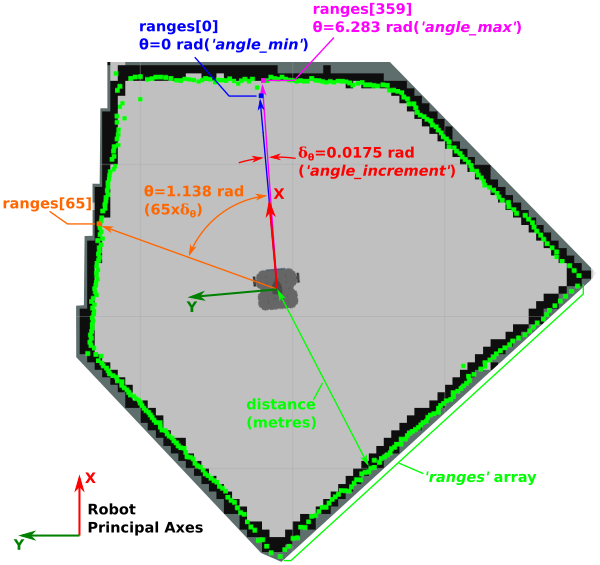
As illustrated in the figure, we can associate each data-point within the ranges array to an angular position by using the angle_min, angle_max and angle_increment values that are also provided within the LaserScan message. We can use the rostopic echo command to drill down into these elements of the message specifically and find out what their values are:

$ rostopic echo /scan/angle_min -n1
0.0

$ rostopic echo /scan/angle_max -n1
6.28318977356

$ rostopic echo /scan/angle_increment -n1
0.0175019223243

Notice how we were able to access specific variables within the /scan message using rostopic echo here, rather than simply printing the whole thing?

Questions

What does the -n1 option do, and why is it appropriate to use this here?
What do these values represent? (Compare them with the figure above)

The ranges array contains 360 values in total, i.e. a distance measurement at every 1° (an angle_increment of 0.0175 radians) around the robot. The first value in the ranges array (ranges[0]) is the distance to the nearest object directly in front of the robot (i.e. at θ = 0 radians, or angle_min). The last value in the ranges array (ranges[359]) is the distance to the nearest object at 359° (i.e. θ = 6.283 radians, or angle_max) from the front of the robot. ranges[65], for example, would represent the distance to the closest object at an angle of 65° (1.138 radians) from the front of the robot (anti-clockwise), as shown in the figure.

The LaserScan message also contains the parameters range_min and range_max, which represent the minimum and maximum distance (in meters) that the LiDAR sensor can detect, respectively. You can use the rostopic echo command to report these directly too.

Question

What is the maximum and minimum range of the LiDAR sensor? Use the same technique as we used above to find out.

Finally, use the rostopic echo command again to display the ranges portion of the LaserScan topic message. There's a lot of data here (360 data points in fact, as you know from above!) so let's just focus on the data within a 0-65° angular range (again, as illustrated in the figure). You can therefore use the rostopic echo command as follows:

rostopic echo /scan/ranges[0:65] -c

We're dropping the -n1 option now, so that we can see the data points updating in real-time, but we're introducing the -c option to clear the screen after every message to make things a bit clearer. You might need to expand the terminal window so that you can see all the data points; data will be bound by square brackets [], and there should be a --- at the end of each message too, to help you confirm that you are viewing the whole thing.

The main thing you'll notice here is that there's lots of information, and it changes rapidly! As you have already seen though, it is the numbers that are flying by here that are represented by red dots in RViz. Head back to the RViz screen to have another look at this now. As you'll no doubt agree, this is a much more useful way to visualise the ranges data, and illustrates how useful RViz can be for interpreting what your robot can see in real-time.

What you may also notice is several inf values scattered around the array. These represent sensor readings that are outside the sensor's measurement range (i.e. greater than range_max or less than range_min), so the sensor can't report a distance measurement in such cases.

Note

This behaviour is different on the real robots! See Fact-Finding Mission 4 for further info, and be aware of this when developing code for real robots!!

Stop the rostopic echo command from running in the terminal window by entering Ctrl+C.

Simultaneous Localisation and Mapping (SLAM)¶

In combination, the data from the LiDAR sensor and the robot's odometry (the robot pose specifically) are really powerful, and allow some very useful conclusions to be made about the environment a robot is operating within. One of the key applications of this data is "Simultaneous Localisation and Mapping", or SLAM. This is a tool that is built into ROS, and allows a robot to build up a map of its environment and locate itself within that map at the same time! You will now learn how easy it is to leverage this in ROS.

Exercise 2: Building a map of an environment with SLAM¶

Close down all ROS processes that are running now by entering Ctrl+C in each terminal:
1. The Gazebo processes in TERMINAL 1.
2. The RViz processes running in TERMINAL 2.
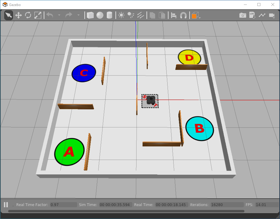
We're going to launch our robot into another new simulated environment now, which we'll be creating a map of using SLAM! To launch the simulation enter the following command in TERMINAL 1:

TERMINAL 1:
```
roslaunch tuos_simulations nav_world.launch
```
The environment that launches should look like this:
Now we will launch SLAM to start building a map of this environment. In TERMINAL 2, launch SLAM as follows:

TERMINAL 2:
```
roslaunch turtlebot3_slam turtlebot3_slam.launch
```
This will launch RViz again, and you should be able to see a model of your TurtleBot3 from a top-down view, this time with green dots representing the real-time LiDAR data. The SLAM tools will already have begun processing this data to start building a map of the boundaries that are currently visible to your robot based on its position in the environment.
In TERMINAL 3 launch the turtlebot3_teleop_key node (you should know how to do this by now). Re-arrange and re-size your windows so that you can see Gazebo, RViz and the turtlebot3_teleop_key terminal instances all at the same time:
Drive the robot around the arena slowly, using the turtlebot3_teleop_key node, and observe the map being updated in the RViz window as you do so. Drive the robot around until a full map of the environment has been generated.
As you're doing this you need to also determine the centre coordinates of the four circles (A, B, C & D) that are printed on the arena floor. Drive your robot into each of these circular zones and stop the robot inside them. As you should remember from Part 2, we can determine the position (and orientation) of a robot in its environment from its odometery, as published to the /odom topic. In Part 2 Exercise 2 you built an odometry subscriber node, so you could launch this now (in a new terminal: TERMINAL 4), and use this to inform you of your robot's x and y position in the environment when located within each of the zone markers:

TERMINAL 4:
```
rosrun part2_navigation odom_subscriber.py
```
Record the zone marker coordinates in a table such as the one below (you'll need this information for the next exercise).

Zone X Position (m) Y Position (m)

START 0.5 -0.04

A

B

C

D
Once you've obtained all this data, and you're happy that your robot has built a complete map of the environment, you then need to save this map for later use. We do this using a ROS map_server package. First, stop the robot by pressing S in TERMINAL 3 and then enter Ctrl+C to shut down the turtlebot3_teleop_key node.
Then, remaining in TERMINAL 3, navigate to the root of your part2_navigation package directory and create a new folder in it called maps:

TERMINAL 3:
```
roscd part2_navigation
```
```
mkdir maps
```
Navigate into this new directory:

TERMINAL 3:
```
cd maps/
```
Then, run the map_saver node from the map_server package to save a copy of your map:

TERMINAL 3:
```
rosrun map_server map_saver -f {map name}
```
Replacing {map name} with a name of your choosing.

This will create two files: a {map name}.pgm and a {map name}.yaml file, both of which contain data related to the map that you have just created. The .pgm file contains an Occupancy Grid Map (OGM), which is used for autonomous navigation in ROS. Have a look at the map by launching it in an Image Viewer Application called eog:

TERMINAL 3:
```
eog {map name}.pgm
```
A new window should launch containing the map you have just created with SLAM and the map_saver node:

White regions represent the area that your robot has determined is open space and that it can freely move within. Black regions, on the other hand, represent boundaries or objects that have been detected. Any grey area on the map represents regions that remain unexplored, or that were inaccessible to the robot.
Compare the map generated by SLAM to the real simulated environment. In a simulated environment this process should be pretty accurate, and the map should represent the simulated environment very well (unless you didn't allow your robot to travel around and see the whole thing!) In a real environment this is often not the case.
Questions
- How accurately did your robot map the environment?
- What might impact this when working in a real-world environment?
Close the image using the button on the right-hand-side of the eog window.

Summary of SLAM¶

See how easy it was to map an environment in the previous exercise? This works just as well on a real robot in a real environment too (as you will observe in one of the Real Waffle "Getting Started Exercises" for Assignment #2).

This illustrates the power of ROS: having access to tools such as SLAM, which are built into the ROS framework, makes it really quick and easy for a robotics engineer to start developing robotic applications on top of this. Our job was made even easier here since we used some packages that had been pre-made by the manufacturers of our TurtleBot3 Robots to help us launch SLAM with the right configurations for our exact robot. If you were developing a robot yourself, or working with a different type of robot, then you might need to do a bit more work in setting up and tuning the SLAM tools to make them work for your own application.

As mentioned above, the map that you created in the previous exercise can now be used by ROS to autonomously navigate the mapped area. We'll explore this now.

Exercise 3: Navigating an Environment Autonomously¶

Close down all ROS processes now so that nothing is running (but leave all the terminal windows open).
In order to perform autonomous navigation we now need to activate a number of ROS libraries, our simulated environment and also specify some custom parameters, such as the location of our map file. The easiest way to do all of this in one go is to create a launch file.
You may have already created a launch directory in your part2_navigation package, but if you haven't then do this now:

TERMINAL 1:
```
roscd part2_navigation
```
```
mkdir launch
```
Next, navigate into this directory and create a new file called navigation.launch:

TERMINAL 1:
```
cd launch/
```
```
touch navigation.launch
```

Open up this file in VS Code and copy and paste the following content:

<!-- Adapted from the Robotis "turtlebot3_navigation" package: 
https://github.com/ROBOTIS-GIT/turtlebot3/blob/master/turtlebot3_navigation/launch/turtlebot3_navigation.launch
-->
<launch>
  <include file="$(find tuos_simulations)/launch/nav_world.launch" />

  <!-- To be modified -->
  <arg name="map_file" default=" $(find part2_navigation)/maps/{map name}.yaml"/>
  <arg name="initial_pose_x" default="0.0"/>
  <arg name="initial_pose_y" default="0.0"/>

  <!-- Other arguments -->
  <arg name="initial_pose_a" default="0.0"/>
  <arg name="model" default="$(env TURTLEBOT3_MODEL)" doc="model type [burger, waffle, waffle_pi]"/>
  <arg name="move_forward_only" default="false"/>

  <!-- Turtlebot3 Bringup -->
  <include file="$(find turtlebot3_bringup)/launch/turtlebot3_remote.launch">
    <arg name="model" value="$(arg model)" />
  </include>

  <!-- Map server -->
  <node pkg="map_server" name="map_server" type="map_server" args="$(arg map_file)"/>

  <!-- AMCL -->
  <include file="$(find turtlebot3_navigation)/launch/amcl.launch">
    <arg name="initial_pose_x" value="$(arg initial_pose_x)"/>
    <arg name="initial_pose_y" value="$(arg initial_pose_y)"/>
    <arg name="initial_pose_a" value="$(arg initial_pose_a)"/>
  </include>

  <!-- move_base -->
  <include file="$(find turtlebot3_navigation)/launch/move_base.launch">
    <arg name="model" value="$(arg model)" />
    <arg name="move_forward_only" value="$(arg move_forward_only)"/>
  </include>

  <!-- rviz -->
  <node pkg="rviz" type="rviz" name="rviz" required="true"
    args="-d $(find turtlebot3_navigation)/rviz/turtlebot3_navigation.rviz"/>

</launch>

Edit the default values in the three lines below the  line:
1. Change {map name} to the name of your map file as created in the previous exercise (remove the {}s!).
2. Change the initial_pose_x and initial_pose_y default values. Current these are both set to "0.0", but they need to be set to match the coordinates of the start zone of the tuos_simulations/nav_world environment (we may have given you a clue about these in the table earlier!)
Once you've made these changes, save the file and then launch it:

TERMINAL 1:
```
{BLANK} part2_navigation navigation.launch
```
Fill in the Blank!

Which ROS command do we use to execute launch files?
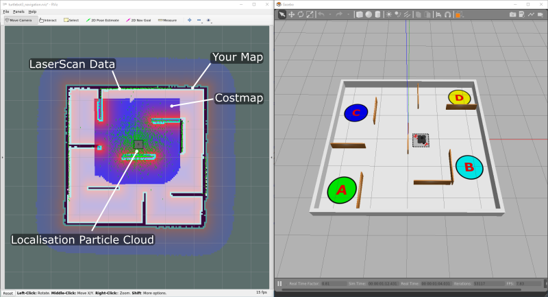
RViz and Gazebo should be launched, both windows looking something like this:

Question

How many nodes were actually launched on our ROS Network by executing this launch file?

As shown in the figure, in RViz you should see the map that you generated with SLAM earlier.
- There should be a "heatmap" surrounding your robot and a lot of green arrows scattered all over the place.
- The green arrows represent the localisation particle cloud, and the fact that these are all scattered across quite a wide area at the moment indicates that there is currently a great deal of uncertainty about the robot's actual pose within the environment. Once we start moving around this will improve and the arrows will start to converge more closely around the robot.
  
  This is actually called a "costmap", and it illustrates what the robot perceives of its environment: blue regions representing safe space that it can move around in; red regions representing areas where it could collide with an obstacle.
- Finally, the green dots illustrate the real-time LaserScan data coming from the LiDAR sensor, as we saw earlier. This should be nicely overlaid on top of the boundaries in our map.
To send a navigation goal to our robot we need to issue a request to the move_base action server. We will cover ROS Actions later in this course, but for now, all you really need to know is that we can send a navigation goal by publishing a message to a topic on the ROS network. In TERMINAL 2 run rostopic list and filter this to show only topics related to /move_base:

TERMINAL 2:
```
rostopic list | grep /move_base
```
This will provide quite a long list, but right at the bottom you should see the item /move_base_simple/goal. We'll use this to publish navigation goals to our robot to make it move autonomously using the ROS Navigation Stack.

Running rostopic info on this topic will allow us to find out more about it:

TERMINAL 2:

rostopic info move_base_simple/goal

Type: geometry_msgs/PoseStamped

Publishers:
  * /rviz (http://localhost:#####/)

Subscribers:
  * /move_base (http://localhost:#####/)
  * /rviz (http://localhost:#####/)

Question

What type of message does this topic use, and which ROS package does it live within?

Run another command now to find out what the structure of this message is (you did this earlier for the LaserScan messages published to the /scan topic).
Knowing all this information now, we can use the rostopic pub command to issue a navigation goal to our robot, via the /move_base_simple/goal topic. This command works exactly the same way as it did when we published messages to the /cmd_vel topic in Part 2 (when we made the robot move at a velocity of our choosing).

Remember that the rostopic pub command takes the following format:
```
rostopic pub {topic_name} {message_type} {data}
```
...but to make life easier, we can use the autocomplete functionality in our terminal to help us format the message correctly:
```
rostopic pub {topic_name} {message_type}[SPACE][TAB]
```
Do this now, (replacing {topic_name} and {message_type} accordingly) to generate the full message structure that we will use to send the navigation goal to the robot, from the terminal. Don't press Enter yet though, as we will need to edit the message data in order to provide a valid navigation goal.
There are four things in this message that need to be changed before we can publish it:
1. frame_id: '' should be changed to frame_id: 'map'
2. The pose.orientation.w value needs to be changed to 1.0:
```
pose:
  orientation:
    w: 1.0
```
3. The pose.position.x and pose.position.y parameters define the location, in the environment, that we want the robot to move to, as determined in the previous exercise:
```
pose:
  position:
    x: {desired location in x}
    y: {desired location in y}
```
  Scroll back through the message using the left arrow key on your keyboard (←), and modify the four parameters of the message accordingly, setting your x and y coordinates to make the robot move to any of the four marker zones in the environment.
Once you're happy, hit Enter and watch the robot move on its own to the location that you specified!

Notice how the green particle cloud arrows very quickly converge around the robot as it moves around? This is because the robot is becoming more certain of it's pose (its position and orientation) within the environment as it compares the boundaries its LiDAR sensor can actually see with the boundaries marked out in the map that you supplied to it.
Have a go at requesting more goals by issuing further commands in the terminal (using rostopic pub) to make the robot move between each of the four zone markers.

Summary¶

We have just made a robot move by issuing navigation goals to an Action Server on our ROS Network. You will learn more about ROS Actions later on in this course, where you will start to understand how this communication method actually works. You will also learn how to create Action Client Nodes in Python, so that - in theory - everything that you have been doing on the command-line in this exercise could be done programmatically instead.

As you have observed in this exercise, in order to use ROS navigation tools to make a robot move autonomously around an environment there are a few important things that we need to provide to the Navigation Stack:

A map of the environment that we want to navigate around.
This means that our robot needs to have already explored the environment once beforehand to know what the environment actually looks like. We drove our robot around manually in this case but, often, some sort of basic exploratory behaviour would be required in the first instance so that the robot can safely move around and create a map (using SLAM) without crashing into things! You will learn more about robotic search/exploration strategies in your lectures.
The robot's initial location within the environment.
...so that it could compare the map file that we supplied to it with what it actually observes in the environment. If we didn't know where the robot was to begin with, then some further exploration would be required to start with, in order for the robot to build confidence in its actual pose in the environment, prior to navigating it.
The coordinates of the places we want to navigate to.
This may seem obvious, but it's an extra thing that we need to establish before we are able to navigate autonomously.

Wrapping Up¶

Odometry data is determined by dead-reckoning and control algorithms based on this alone will be subject to drift and accumulated error.

Ultimately then, a robot needs additional information to pinpoint its precise location within an environment, and thus enhance its ability to navigate effectively and avoid crashing into things!

This additional information can come from a LiDAR sensor, which you learnt about in this session. We explored where this data is published, how we access it, and what it tells us about a robot's immediate environment. We then looked at some ways odometry and laser displacement data can be combined to perform advanced robotic functions such as the mapping of an environment and the subsequent navigation around it. This is all complicated stuff but, using ROS, we can leverage these tools with relative ease, which illustrates just how powerful ROS can be for developing robotic applications quickly and effectively without having to re-invent the wheel!

WSL-ROS Managed Desktop Users: Save your work!¶

Remember, the work you have done in the WSL-ROS environment during this session will not be preserved for future sessions or across different University machines automatically! To save the work you have done here today you should now run the following script in any idle WSL-ROS Terminal Instance:

wsl_ros backup

This will export your home directory to your University U:\ Drive, allowing you to restore it on another managed desktop machine the next time you fire up WSL-ROS.

Part 3: SLAM & Autonomous Navigation

Introduction¶

Aims¶

Intended Learning Outcomes¶

Quick Links¶

Getting Started¶

Laser Displacement Data and The LiDAR Sensor¶

Exercise 1: Using RViz to Visualise Robot Data¶

Interpreting `/LaserScan` Data¶

Simultaneous Localisation and Mapping (SLAM)¶

Exercise 2: Building a map of an environment with SLAM¶

Summary of SLAM¶

Advanced Navigation Methods¶

Exercise 3: Navigating an Environment Autonomously¶

Summary¶

Further Reading¶

Wrapping Up¶

WSL-ROS Managed Desktop Users: Save your work!¶

Zone	X Position (m)	Y Position (m)
START	0.5	-0.04
A
B
C
D

Part 3: SLAM & Autonomous Navigation

Introduction¶

Aims¶

Intended Learning Outcomes¶

Quick Links¶

Getting Started¶

Laser Displacement Data and The LiDAR Sensor¶

Exercise 1: Using RViz to Visualise Robot Data¶

Interpreting /LaserScan Data¶

Simultaneous Localisation and Mapping (SLAM)¶

Exercise 2: Building a map of an environment with SLAM¶

Summary of SLAM¶

Advanced Navigation Methods¶

Exercise 3: Navigating an Environment Autonomously¶

Summary¶

Further Reading¶

Wrapping Up¶

WSL-ROS Managed Desktop Users: Save your work!¶

Interpreting `/LaserScan` Data¶